Linear Regression Single Variable in Python

In this article we will look at what is simple linear regression, the math behind it and then see hands-on implementation of simple linear regression in Python language.

 

Let’s see how to predict home prices using a machine learning technique called simple linear regression. By simple we mean single variable regression. Regression is a supervised learning technique which is used for making predictions.

 

Here, single variable means there is only one independent variable (you will see what is independent variable later). For example predicting the price of a house based on the area of house. Given below is a sample of data showing area of the house and corresponding price for houses in Monroe, New Jersey, USA.

 

Area	Price
2600	550000
3000	565000
3200	610000
3600	680000
4000	725000

 

Introduction to Linear Regression

Using this data (in the above table) we will build a model/function that can tell us the prices of the homes whose are is 3300 sq.ft. and 5000 sq.ft. We can plot the above data as a scatter plot (we will see the python code later) as shown below. Download the dataset.

 

 

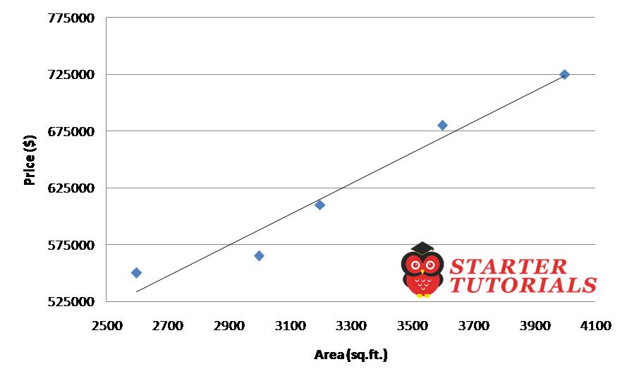
The blue points in the above figure represent the price of the house for a given area. The black line which is going through the data points (some of them) is the one which best fits the given data. It is also called the regression line. We will see how to get that line using Python code later.

 

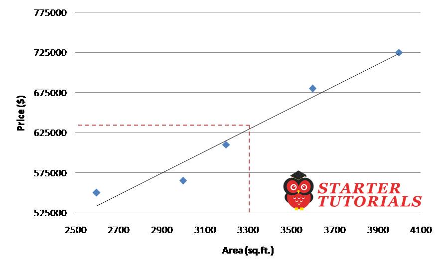
Once we get the line, we can predict the price of a new house with a given area. For example, the price of a house whose area is 3300 sq.ft., its price will be 628715$.

 

 

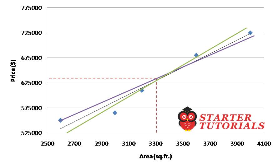
Now you might be thinking how did we get the black line (regression line)? The line is not clearly going through (touching) all the data points and there are number of ways we can draw the lines, green and violet, as shown below.

 

 

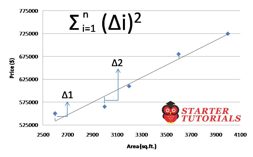
How to find the best fit (line) is, we calculate delta, which is the an error between the actual data point and the line (as shown in below figure)  which is predicted by the linear equation. We square the individual errors and sum them up and we try to minimize those. So we repeat this process for different lines and come up with the best line that has the least value for the sum of squared errors.

 

 

From your elementary school or high school math you might have remembered the equation of a line which is shown below.

 

 

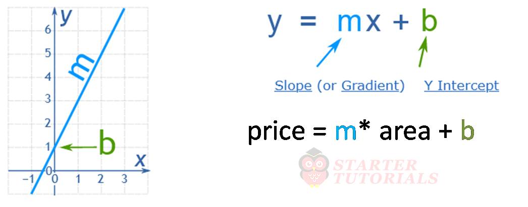
In our house prices example, the variable y in the line equation is the price of the house and the variable x is area of the house. Area is called an independent variable (generally the variable on x-axis) and price is called a dependent variable (generally the variable on y-axis) because we are calculating the price based on area.

 

Linear Regression Single Variable in Python

Now we will see linear regression in action using Python. The hands-on will be done using Jupyter Notebook. I hope you already have some experience with it and Python programming language. First we will import some important libraries.

 

import pandas as pd
import numpy as np
import matplotlib.pyplot as plt
from sklearn import linear_model

 

NumPy and Pandas libraries are used to load and perform operations on the data. Matplotlib library is used to plot graphs. Sklearn or also called scikit-learn is used here to build our model. First, we will load our dataset using Pandas.

 

df = pd.read_csv("house_prices.csv")

 

Here, read_csv is a method used to load our dataset in the file house_prices.csv. It returns back a dataframe which is stored in df variable. Now, we will plot a scatter plot to see the distribution of our house prices data.

 

plt.xlabel("Area(sq.ft.)")
plt.ylabel("Price($)")
plt.scatter(df.Area, df.Price)

 

If you run the above line you should see a scatter plot like below.

 

 

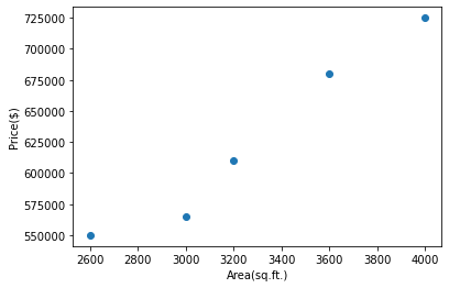
From the above figure we can see that the distribution is approximately linear and we can use linear regression. First we need to create an object of LinearRegression. Now we will fit our data using fit method. Fitting the data means we are training the linear regression model using the available data in our dataset.

 

reg = linear_model.LinearRegression()
reg.fit(df[['Area']], df.Price)

 

The first argument for the fit method is the independent variable and the second argument will be the dependent variable. Once we execute the above code, linear regression model will fit our data and will be ready to predict the price of houses for given data.

 

Now, let’s try to predict the price of house with area as 3300 sq.ft. The code for that is:

 

reg.predict([[3300]])

 

The predicted price is:

 

628715.75342466

 

Now let’s look at the internal details how linear regression was able to predict the above value. Linear regression while fitting the data will calculate the coefficient or slope and intercept i.e., m and b.

 

We can see the value of m or coefficient by writing reg.coef_ and we get the value 135.78767123. Similarly we can see the value of b or intercept by writing reg.intercept_ and we get the value 180616.43835616432. You can verify by calculating 135.78767123 * 3300 + 180616.43835616432 gives 628715.75342466.

 

Let’s try to predict the house price for 5000 sq.ft. by writing reg.predict([[5000]). We will get the predicted price as 859554.79452055.

 

Now let’s see the linear regression line on our scatter plot. For that we need to add another line in Python as shown below.

 

plt.xlabel("Area(sq.ft.)")
plt.ylabel("Price($)")
plt.scatter(df.Area, df.Price)
plt.plot(df.Area, reg.predict(df[['Area']]), color='blue')

 

When we execute the above piece of code, we can see the regression line as shown below.

 

 

Exercise on Linear Regression with Single Variable

So, let’s try out an exercise. First download Canada’s per capita income dataset. The data in the CSV file is as shown below.

 

year	pci
1970	3399.299037
1971	3768.297935
1972	4251.175484
1973	4804.463248
1974	5576.514583
1975	5998.144346
1976	7062.131392
1977	7100.12617
1978	7247.967035
1979	7602.912681
1980	8355.96812
1981	9434.390652
1982	9619.438377
1983	10416.53659
1984	10790.32872
1985	11018.95585
1986	11482.89153
1987	12974.80662
1988	15080.28345
1989	16426.72548
1990	16838.6732
1991	17266.09769
1992	16412.08309
1993	15875.58673
1994	15755.82027
1995	16369.31725
1996	16699.82668
1997	17310.75775
1998	16622.67187
1999	17581.02414
2000	18987.38241
2001	18601.39724
2002	19232.17556
2003	22739.42628
2004	25719.14715
2005	29198.05569
2006	32738.2629
2007	36144.48122
2008	37446.48609
2009	32755.17682
2010	38420.52289
2011	42334.71121
2012	42665.25597
2013	42676.46837
2014	41039.8936
2015	35175.18898
2016	34229.19363

 

In the above dataset we have data up to the year 2016. So, let’s use our dataset and try to predict the per capita income for the year 2021. The code and scatter plot along with the linear regression’s line is shown below.

 

df1 = pd.read_csv("canada_pci.csv")

plt.xlabel("Year")
plt.ylabel("Per Capita Income")
plt.scatter(df1.year, df1.pci)

reg1 = linear_model.LinearRegression()
reg1.fit(df1[['year']], df1.pci)

reg1.predict([[2021]])

plt.xlabel("Year")
plt.ylabel("Per Capita Income")
plt.scatter(df1.year, df1.pci)
plt.plot(df1.year, reg1.predict(df1[['year']]), color='red')

 

 

The result of reg1.predict([[2021]]) is 42117.15916964i.

 

That’s it for this tutorial on linear regression single variable in Python language. If you have any questions or if there are any corrections, please comment below.

 

For more information, visit the following links:

• Machine Learning Tutorial Python – 2: Linear Regression Single Variable