Gradient Descent and Cost Function in Python

In this article we are going to look at gradient descent and cost function in Python programming language.

 

Mean Squared Error (MSE)

In our school days we used to solve linear equations. For example consider the linear equation y=2x+3. For given x values, [1,2,3,4,5] we can calculate y values as [5,7,9,11,13].

 

However, in case of machine learning we have the values of x and y already available with us and using them we have to derive a linear equation. The equation is also known as prediction function. We can use the prediction function to calculate the future value of y.

 

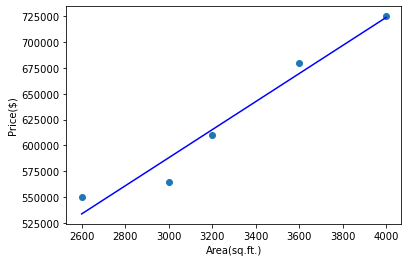
In our earlier simple linear regression tutorial, we have used the following data to predict the house prices:

 

Area	Price
2600	550000
3000	565000
3200	610000
3600	680000
4000	725000

 

The linear equation we got while implementing linear regression in Python is:

 

So, our goal today is to determine how to get the above equation. This equation is nothing but the line which best fits the given data as shown below.

 

 

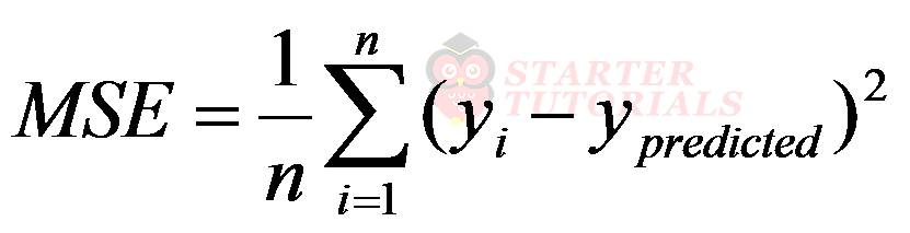
Coming up with the best fit line and the linear equation is to calculate the sum of squared errors as already discussed in our simple linear regression tutorial. We divide the sum of squared errors with the number of data points n. The result we get is called Mean Squared Error (MSE). The formula for MSE is:

 

 

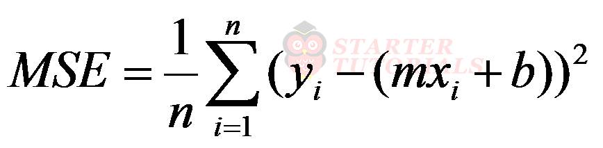
The mean squared error is also called a cost function. There are other cost functions as well but MSE is the popular one. In the above equation we will expand ypredicted as shown below:

 

 

Now we can toss various values for m and b and see which values will give least MSE value. Such a brute force method is inefficient. We need another approach which will give the optimum values for m and b in a few steps.

 

Gradient Descent Algorithm

 

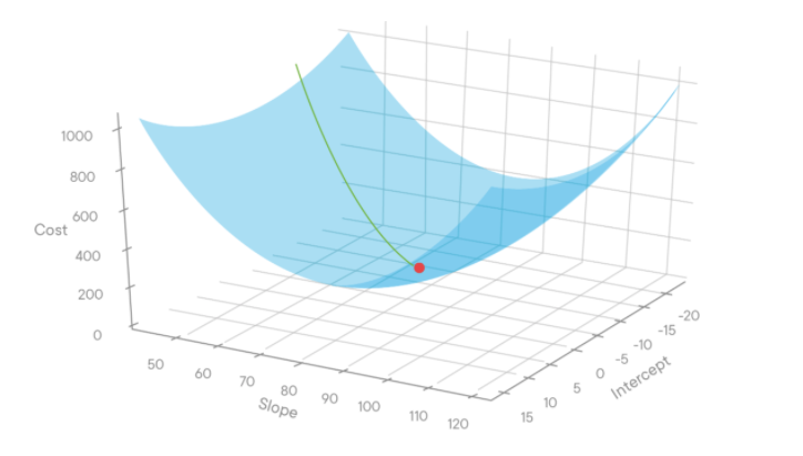
If we plot a 3D graph for some value for m (slope), b (intercept), and cost function (MSE), it will be as shown in the below figure.

 

Source: miro.medium.com

 

In the above figure, intercept is b, slope is m and cost is MSE. If we plot the cost for various values of m and b, we will get the graph as shown above. Generally people start with the initial values of m=0 and b=0. The corresponding cost will be the starting point of the red line (at the top) as shown above.

 

Then we reduce the values of m and b (a step) and again calculate the cost. We repeat this process of steps until we get the minimum cost (the red dot in the above figure). Then we take the corresponding values of m and b for getting the linear equation.

 

When we look at the above 3D graph with b x-axis and m as x-axis, the graphs will be as shown below.

 

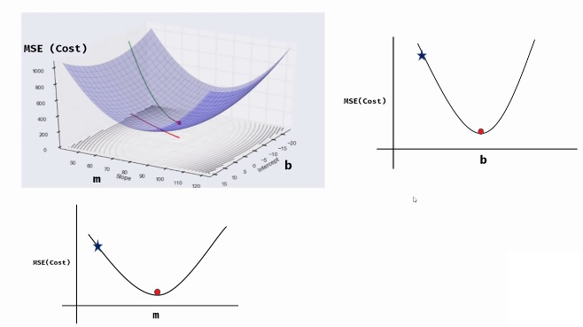
Source: youtube.com

 

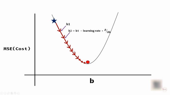
Let’s consider the values of b. We generally start at some random initial value. Let’s say we are decreasing the value of b (steps) by a constant value. In such case, we might miss the optimum value (also called global minima) of b (red dot) as shown in below figure.

 

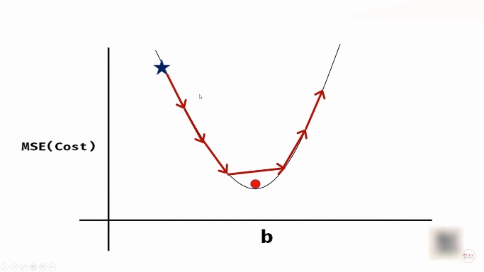
Source: youtube.com

 

If we decrease the value of b so that it follows the curvature in the graph, we can reach the optimum value of b as shown below.

 

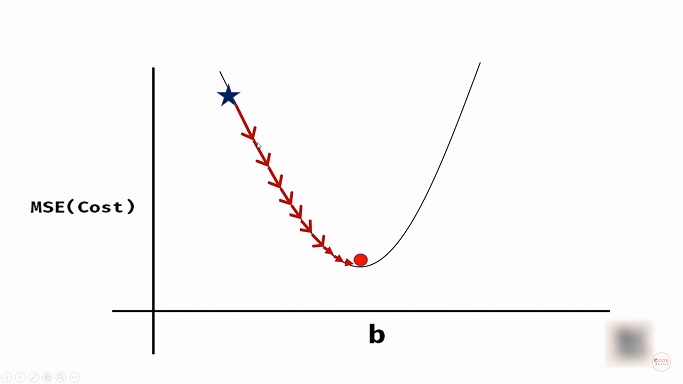
Source: youtube.com

 

So, how do we follow the curvature? At each step we have to calculate the slope of the tangent (dashed-line in below figure) and use something called learning rate to approach at the next value of b.

 

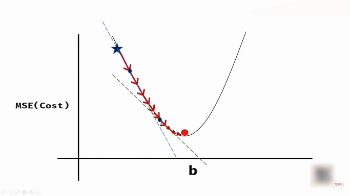
Source: youtube.com

 

To calculate the slope of a line at a particular point we need the concepts of derivatives and partial derivatives (calculus). Those concepts will not be covered here. So, we are directly going to jump into the equations as shown below.

 

 

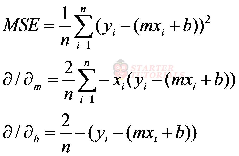
Now as we got the slope (partial derivatives given above), we need to calculate the step (next value) which uses learning rate. So, for taking the next step, the equations are as given below.

 

 

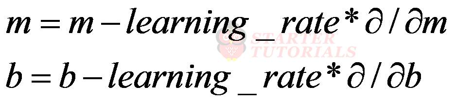
For example, updating the value of b will look as shown below.

 

Source: youtube.com

 

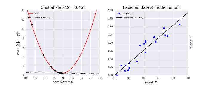
The gradient descent algorithm in action looks something like as shown in the below animation.

 

 

Gradient Descent and Cost Function in Python

Now, let’s try to implement gradient descent using Python programming language. First we import the NumPy library for arrays purpose as they are easy when compared to Python lists. Then we define a function for implementing gradient descent as shown below.

 

import numpy as np

def gradient_descent(x, y):
    #initial value of m and b
    m_curr = b_curr = 0
    #initialize number of steps
    iterations = 1000
    #Number of data points n
    n = len(x)
    #Initialize learning rate
    learning_rate = 0.001
    
    for i in range(iterations):
        y_pred = m_curr * x + b_curr
        cost = (1/n) * sum([val**2 for val in (y-y_pred)])
        md = -(2/n)*sum(x*(y-y_pred))
        bd = -(2/n)*sum(y-y_pred)
        m_curr = m_curr - learning_rate * md
        b_curr = b_curr - learning_rate * bd
        print("m {}, b {}, cost {}, iteration {}".format(m_curr, b_curr, cost, i))

 

In the above code we are just trying out some values for m_curr, b_curr, iterations and learning_rate. Now, we execute our function with the following code.

 

x = np.array([1,2,3,4,5])
y = np.array([5,7,9,11,13])

gradient_descent(x, y)

 

The output (modified) for the above code is given below.

 

m 0.062, b 0.018000000000000002, cost 89.0, iteration 0
m 0.122528, b 0.035592000000000006, cost 84.881304, iteration 1
m 0.181618832, b 0.052785648000000004, cost 80.955185108544, iteration 2
m 0.239306503808, b 0.069590363712, cost 77.21263768455901, iteration 3
m 0.29562421854195203, b 0.086015343961728, cost 73.64507722605434, iteration 4
m 0.35060439367025875, b 0.10206956796255283, cost 70.2443206760065, iteration 5
m 0.40427867960173774, b 0.11776180246460617, cost 67.00256764921804, iteration 6
m 0.4566779778357119, b 0.13310060678206653, cost 63.912382537082294, iteration 7
m 0.5078324586826338, b 0.14809433770148814, cost 60.966677449199324, iteration 8
m 0.5577715785654069, b 0.16275115427398937, cost 58.15869595270883, iteration 9
m 0.606524096911324, b 0.17707902249404894, cost 55.481997572035766, iteration 10
....
m 2.4499152007487943, b 1.3756633674836414, cost 0.4805725141922505, iteration 991
m 2.449763086127419, b 1.3762125495441813, cost 0.4802476096343826, iteration 992
m 2.4496110229353505, b 1.3767615459283284, cost 0.4799229247373742, iteration 993
m 2.4494590111552026, b 1.3773103566988596, cost 0.47959845935271794, iteration 994
m 2.449307050769595, b 1.3778589819185307, cost 0.47927421333200615, iteration 995
m 2.449155141761153, b 1.3784074216500761, cost 0.47895018652693155, iteration 996
m 2.449003284112507, b 1.3789556759562092, cost 0.4786263787892881, iteration 997
m 2.448851477806295, b 1.3795037448996217, cost 0.4783027899709678, iteration 998
m 2.448699722825159, b 1.3800516285429847, cost 0.47797941992396514, iteration 999

 

From the above output we can see that the cost in the last iteration is still reducing. So, we can increase the number of iterations or change the learning rate to get the least cost.

 

Generally we will start with less number of iterations and start with a higher learning rate, say, 0.1 and see the output values. From here onwards we will just change the learning rate and number of iterations (trial and error) to get the minimum cost.

 

When you run the above function with learning_rate as 0.08 and iterations as 10000, you can see that we will get the m value as 2 (approx.) and b value as 3 (approx.) which are the expected values. So, the linear equation is          y = 2x + 3.

 

Now its time for an exercise.

 

Exercise on Gradient Descent and Cost Function

We are going to work on a dataset which contains student test scores of mathematics (math) and computer science (cs) subjects. We have to find the correlation (some kind of dependency) between the math and cs subjects. Download the test scores dataset. The data is shown below.

 

name	math	cs
david	92	98
laura	56	68
sanjay	88	81
wei	70	80
jeff	80	83
aamir	49	52
venkat	65	66
virat	35	30
arthur	66	68
paul	67	73

 

So, for this exercise we will consider the math values as input  or x and cs  values as the output or y. The code for gradient descent will be as shown below.

 

import numpy as np
import pandas as pd
import math

df = pd.read_csv("test_scores.csv")

def gradient_descent2(x, y):
    #initial value of m and b
    m_curr = b_curr = 0
    #initialize number of steps
    iterations = 1000000
    #Number of data points n
    n = len(x)
    #Initialize learning rate
    learning_rate = 0.0002
    
    cost_previous = 0
    
    for i in range(iterations):
        y_pred = m_curr * x + b_curr
        cost = (1/n) * sum([val**2 for val in (y-y_pred)])
        md = -(2/n)*sum(x*(y-y_pred))
        bd = -(2/n)*sum(y-y_pred)
        m_curr = m_curr - learning_rate * md
        b_curr = b_curr - learning_rate * bd
        if math.isclose(cost, cost_previous, rel_tol=1e-20):
            break
        cost_previous = cost
        print("m {}, b {}, cost {}, iteration {}".format(m_curr, b_curr, cost, i))

x = np.array(df.math)
y = np.array(df.cs)

gradient_descent2(x, y)

 

In the above program we are using math.isclose method to stop the execution of our gradient descent function when the previous cost is pretty close to the current cost.

 

If we execute the above program we will get m as 1.0177381667793246, b as 1.9150826134339467 and cost as 31.604511334602297 at iteration number 415532.

 

If you want to verify whether the values m and b correct or not, we can use our linear regression model. The code is given below.

 

from sklearn import linear_model

reg = linear_model.LinearRegression()
reg.fit(df[['math']],df.cs)

print(reg.coef_, reg.intercept_)

 

When we execute the above code the values we will get are 1.01773624 and 1.9152193111569176. These values are pretty close to what we got earlier.

 

That’s it folks! I hope you enjoyed this tutorial. If you have any questions or suggestions please comment below.

 

For more information visit the following links:

• Machine Learning Tutorial Python – 4: Gradient Descent and Cost Function